Understanding Window Functions in SQL Server

In the realm of database operations, while regular aggregate functions dominate by working on entire tables through the GROUP BY clause, a less-explored yet highly potent tool exists—the window functions. Operating on a set of rows, these functions yield a distinct aggregated value for each row. What sets them apart? Unlike regular aggregate functions, window functions don't collapse rows into a single output; each row retains its identity, enriched with an aggregated value.

The Advantage of Window Functions

Consider this: you're analyzing sales data and need to calculate the total sales for each day while retaining the details of individual transactions. Here's where window functions shine. They maintain the granularity of your data, allowing you to derive insights without sacrificing detail. No need for complex self-joins or cumbersome subqueries; window functions elegantly handle the task at hand.

How Window Functions Work

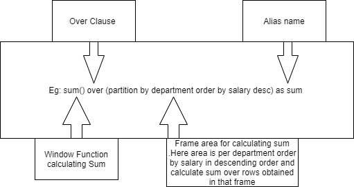
Window functions operate within a defined window of rows, specified using the OVER clause. This window can be partitioned and ordered according to your requirements. The function then computes a value for each row based on the data within this window, without altering the original row structure

Syntax for Window Functions

In a simple expression, a window function looks like this:

function(expression|column) OVER(
    [PARTITION BY expr_list optional] [ORDER BY order_list optional])

Let's go over the syntax piece by piece:

function(expression|column) is the window function such as SUM() or RANK().

OVER() specifies that the function before it is a window function not an ordinary one. So when the SQL engine sees the over clause it will know that the function before the over clause is a window function.

The OVER() clause has some parameters which are optional depending on what you want to achieve. The first one being PARTITION BY.

The PARTITION BY divides the result set into different partitions/windows. For example if you specify the PARTITION BY clause by a column(s) then the result-set will be divided into different windows of the value of that column(s).

Common Window Functions

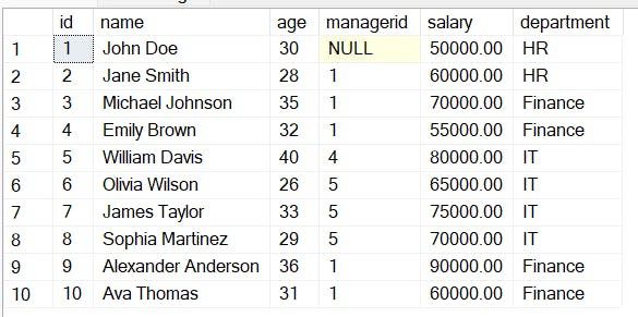
Consider the following table of Employees data:

Syntax for Window functions

Here's an explanation of each common window function:

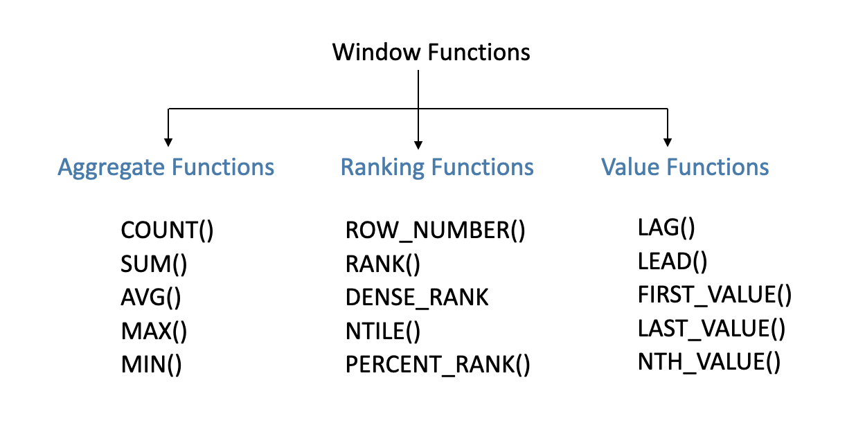
1. ROW_NUMBER(): This function assigns a unique sequential integer to each row within a specified partition. It simply generates a row number for each row, starting from 1.

2. RANK(): Similar to ROW_NUMBER(), RANK() assigns a unique rank to each distinct row within a partition, but it leaves gaps in the ranking when there are ties. For example, if two rows have the same value, they will both receive the same rank, and the next row will receive the rank following the number of tied rows.

3. DENSE_RANK(): DENSE_RANK() is similar to RANK(), but it doesn't leave gaps in the ranking. If two rows have the same value, they both receive the same rank, and the next row receives the next consecutive rank, without any gaps.

4. SUM(), AVG(), MAX(), MIN(): Although these are typically considered aggregate functions, they can also be used as window functions when combined with the OVER() clause. When used in this context, they calculate aggregate values over a specific window of rows rather than the entire table.

SELECT id,name,age,managerid,salary,department
    ,RANK() OVER (ORDER BY salary DESC) AS rank
    ,DENSE_RANK() OVER (ORDER BY salary DESC) AS Dense_rank
    ,row_number() OVER (ORDER BY salary DESC) AS salary_rank
FROM Employees;
--output

In the above query:

• ROW_NUMBER will just assign a unique number to each row based on the descending order of the salary.

• RANK will assign the same rank to employees who have the same salary, and the next rank will skip the number of employees who share that salary(rank 5,8 are skipped in rank column).

• DENSE_RANK employees with the same salary would still get the same rank, but there won't be any gaps in the ranks(similar to rank but it will assign rank without gap).

LEAD() and LAG(): These functions allow you to access data from subsequent (LEAD()) or preceding (LAG()) rows within the partition. For example, you can retrieve the value of the next or previous row without using self-joins or subqueries.

Syntax for LAG

LAG(scalar_expression [, offset [, default ]]) OVER ( [ partition_by_clause ] order_by_clause )

• scalar_expression – The value to be returned based on the specified offset.

• offset – The number of rows back from the current row from which to obtain a value. If not specified, the default is 1.

• default – default is the value to be returned if offset goes beyond the scope of the partition. If a default value is not specified, NULL is returned.

• partition_by_clause: An optional clause that divides the result set into partitions. The LAG() function is applied to each partition separately.

• order_by_clause: The order of the rows within each partition. This is mandatory and must be specified.

SELECT id,name,age,salary,department,
    --retrieves the salary of the previous row ordered by id
    LAG(salary) OVER (ORDER BY id ) AS previous_salary,
    -- retrieves the salary of the next row ordered by id.
    LEAD(salary) OVER (ORDER BY id ) AS next_salary
FROM Employees;

if want to get 0(ZERO) instead of NULL

LAG(salary, 2, 0) OVER (ORDER BY id) AS two_rows_back_salary

LEAD(salary, 2, 0) OVER (ORDER BY id) AS next_to_next_salary

This will provide you with thesalaryvalue from two rows back in the result set, ordered byid, and it will return0if there are not enough preceding rows.

Aggregate window functions

Total salary received within each department by using the SUM window function along with the PARTITION BY clause.

SELECT id,name,age,department,salary,
   SUM(salary) OVER(PARTITION BY department) AS total_salary_received
FROM Employees;

You can use various other aggregate functions such as COUNT, AVG, MIN, and MAX along with the PARTITION BY clause to calculate different metrics within each department. Here's how you can use them:

SELECT id, name,age,department,salary,
    COUNT(*) OVER (PARTITION BY department) AS employee_count,
    AVG(salary) OVER (PARTITION BY department) AS average_salary,
    MIN(salary) OVER (PARTITION BY department) AS min_salary,
    MAX(salary) OVER (PARTITION BY department) AS max_salary
FROM Employees;

Conclusion

In conclusion, window functions in SQL Server offer a versatile and efficient way to perform complex analytical tasks. By operating on a set of rows while preserving their individual identities, these functions provide insights into data relationships and patterns without the need for cumbersome self-joins or subqueries. Leveraging window functions empowers SQL developers to enhance the sophistication and efficiency of their queries, ultimately facilitating more insightful data analysis and decision-making.